Reactive Investing vs Regular Investing

I did this POST a while ago about “Timing the Market” – and the overall summary I came to was that it is incredibly difficult to try and time the market. Often, you are better off just investing regularly and get that time in the market, as opposed to trying to time the market.

Even though I came to that conclusion, the thought still did not leave my mind though, and I was wondering if there was some way of investing that could be carried out that would provide better returns than simply investing every month for instance.

I have no intention of trying to analyse stocks/ETFs for hours a day and trying to predict gains or falls, so I was looking for a methodology that would only base itself from previous results, that way, I did not need to do any sort of analysis at all. It would be a completely systematic approach where all I would have to look at would be previous results. I do not want any emotion or estimation needed to go into when to buy or sell.

Methodology

This is only my first experiment at something like this, in the future I might see if there is any sort of fine tuning that I can do that will provide me with the results I want. My aim at the start is to keep it simple, trying my best not to over-complicate anything and hopefully not confuse myself more than anything.

Now to get down to it, what did I actually do?

Firstly, I used the SPY ETF initially – I like to use this one a lot of the time because it has longevity (been around since 1993) so it provides a decent history of data.

By looking at the daily value of the ETF, I compare it to the previous day to see the gain/loss it had relative to the previous day.

Buy Trigger – I set up “Buy Trigger” to purchase shares after there was a drop in value – initially I will set this at -2.00% (I will talk about comparing different values later)

Sell Trigger – I also set up a “Sell Trigger” to sell shares after there was a rise in value – initially I will set this at +3.70% (again I will talk about comparing different values later)

The theory with the above is, when the price goes down a bit, it might be at a discounted rate, and if it goes up significantly over a day, it might be at an over-priced amount. That is the theory anyway.

Sell Amount – I didn’t want to automatically sell the entire portfolio if the “Sell Trigger” was reached, so I put in a variable so that only X% of the portfolio was sold when the trigger was reached. I have set this at 60%.

Trade Cost – There could be more or less transactions compared with regular investing, so I have added a trade cost of $10.00 to account for this.

Daily Savings – I have allowed for a daily savings rate of $200.00 for this simulation. I should state however that it is only $200.00 for every day that there are stock prices for. So, for public holiday/weekends when the market was closed, it does not allow for savings over these periods.

Capital Gains Tax Rate – Because I will be selling stocks in one simulation, I needed to account for Capital Gains Tax that will be required to be paid throughout. The spreadsheet keeps track of the “Average Paid Price” and calculates the capital gains earned. I have used a capital gains tax rate of 15.00% initially. I should also mention that there were times when there was a negative capital gains (or a capital loss), this could potentially have tax benefits, but I have not included these in terms of the calculations.

Example

The above might sound relatively confusing, but I will try and explain how it works in practice.

The share price data for the SPY ETF starts on 1/2/1993 where it had a price of $26.154 (I am using adjusted close price for the purposes of my data, to take into account dividends and splits). For reference, the data I am using only goes up to 29/1/2021.

On 12/2/1993 the Adjusted Close price was 26.357. The next day of trading (16/2/1993) the Adjusted Close price was 25.692. This was a -2.52% drop in price, so it hit a “Buy Trigger”, so the $2,000 that had been saved up since the start was used to purchase 77 shares.

On 27/10/1997 the Adjusted Close price was 57.238. On 28/10/1997 the Adjusted Close price was 60.541. This was a 5.77% rise in price, so it hit a “Sell Trigger”. This was the first “Sell Trigger” in the simulation and at this stage the portfolio had amassed 6,556 shares at an average buy price of $36.51.

3,933 shares (60% of 6,556) were sold for $238,095.94. With the total buy price of these shares at $143,594.58 (3,933 x $36.51) for a Capital Gains of $94,501.36. The CGT to be paid for this was $14,175.20 (15% x $94,501.36)

The next “Buy Trigger” was actually achieved on 30/10/1997 (just 2 days after the first Sell Trigger) when the price dropped by 2.21%. On this date 3,803 shares were purchased (as you can see this is less than the 3,933 so it did not work out great, unfortunately CGT did not help and ate into the profits significantly)

The above process was repeated over the next 20 or so years until 29/1/2021.

Base Comparison

To compare the above simulation, I have compared it to a “Regular Investment” which simply accumulates shares, and purchases at the start of every month, regardless of the share value at the time. This model does not sell shares and hence no capital gains tax will need to be paid.

Results

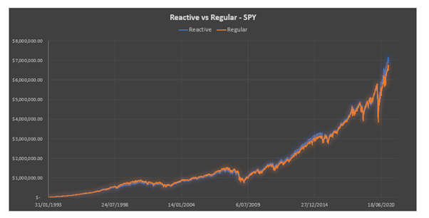
The above graph shows the value of the portfolio in each scenario over time. As you can see they do closely match each other for the most part.

At the end of the simulation each portfolio had the following value:

Reactive Model: $6,893,363.04

Regular Model: $6,515,441.75

That is an added profit of almost $380,000.00 over the investment period. While this is definitely not insignificant and represents a 5.80% improvement in the regular investment return.

The per annum return for the Regular Model is 9.00% (assuming $1,000 per week invested) with the per annum return for the Reactive Model around 9.25% per annum.

Overall, it only brings about a 0.25% improvement in the return, which is better than 0.00% (or less), but I wouldn’t really call it game changing.

Another thing I was hoping to compare was the number of transactions, I was concerned that having significantly more transactions may eat into the profits due to brokerage costs. With these numbers however the number of transactions were as follows

Reactive Model:

Buy Transactions: 295

Sell Transactions: 52

TOTAL Transactions: 347

Regular Model:

TOTAL Transactions: 336

An additional 11 transactions over a 28-year time period are fairly negligible, which is good news.

It is worth noting that the calculations to determine the overall return do consider a $10 brokerage cost for every transaction, so the final value of each portfolio does take into account the number of transactions anyway.

Adjusting Buy or Sell Triggers

Before, I touched briefly on comparing different buy or sell triggers, because I was not sure if there was an optimum value that could be used. Initially I have used a Sell Trigger of 3.70% and a Buy Trigger of -2.00%. But I wanted to be able to compare a wide range of triggers to see what type of results they produced.

Fortunately, since it was just an input value, it was easy to change the variable and see what the results looked like. However, comparing a wide range of values easily did prove to be more difficult. By using a data-table however, I was able to quickly (somewhat, it did take some loading time) to compare different results relatively easily.

The below table provides the difference between Reactive and Regular model using the corresponding Buy and Sell Triggers. The value in the table is in ‘000s as well.

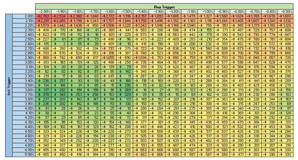
Using conditional formatting has made it somewhat easier to quickly see where the best returns are achieved, as well as where the worst returns are achieved.

As you can see from our example, where we had triggers of 3.70% and -2.00%, it lines up on our table with a return of $378,000 – as we had initially.

If we went with triggers of 2.50% and -1.60%, that would line up with a value of -$488,000, that means our Reactive Model would perform worse than our Regular Model.

From the table above, there is only 56 instances where the Reactive Model outperforms the Regular Model, compared to 440 instances where it underperformed.

Although this does sound like it might fail more often than it succeeds, it is not really the case, because I was more looking for specific “Trigger” levels which might work across a variety of different ETFs, to see if there was a trend that developed over time. Basically, I want to see a positive patch of returns in the same area across a wide range of ETFs.

Comparing Other ETFs

Although the SPY ETF is quite diversified, I wanted to try it on other ETFs to see if I would be able to achieve similar results. At this stage I have only carried out these simulations on the following ETFs:

• VDHG
• VGS
• VAS

It is not an ideal sample size, especially with some overlap between VAS/VGS within VDHG, but if there were trends emerging after looking at these ETFs, then it would encourage me to keep going and seeing if it is a viable investment method.

I will start by using the same triggers as before (3.70% and -2.00%) as well as all the other same inputs and determine what the results do look like.

VDHG Results

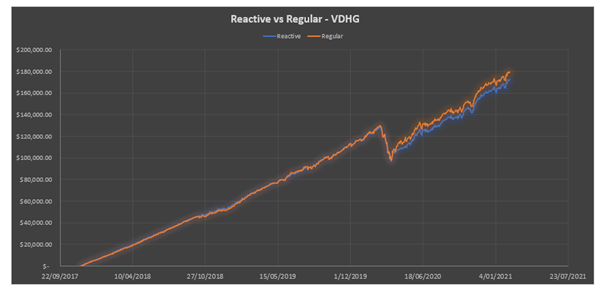
You can see in the above graph that using the default triggers, the Regular Model performs better than the Reactive Model.

In this instance they had the following value at the end of the period:

Reactive Model: $172,038.58

Regular Model: $179,289.19

Keep in mind that this ETF only started in late 2017, so there is not a significant amount of historical data to go from.

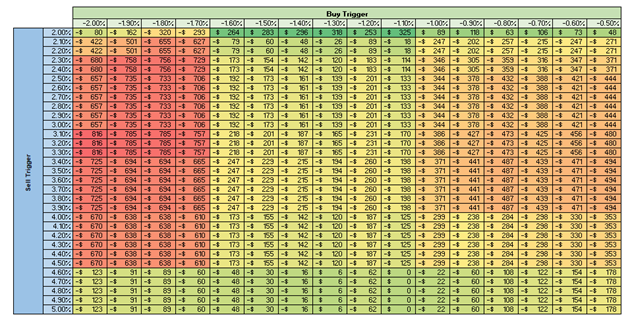
The above shows the results given the different variables of the Buy and Sell Trigger. Note that this time the value shown in the table is in 0s, not 000s as it was in the SPY Table.

While there are some sections of positive returns, there is no overlap with the SPY ETF, which would show Triggers that would work for both ETFs.

VGS Results

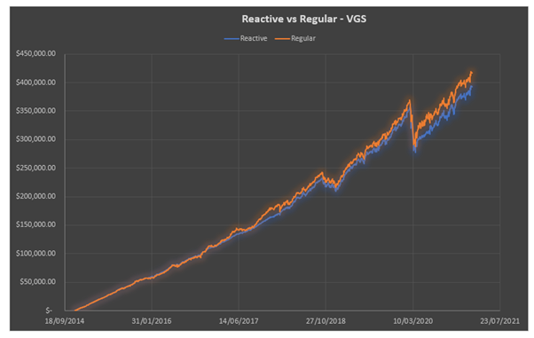
Similar to VDHG, the VGS ETF did not provide a positive result comparing the Reactive Model and the Regular Model.

In this instance they had the following value at the end of the period:

Reactive Model: $392,761.46

Regular Model: $416,979.20

This is a loss of over $24,000 by investing using the Reactive Model compared to the Regular Model.

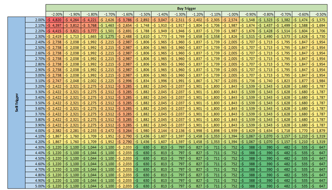
The table above does not show friendly results either, again the results are only in 0s, but there is not once instance which provides positive results.

VAS Results

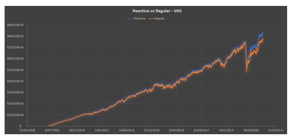
This graph shows somewhat more promising results, with a better return using the Reactive Model compared to the Regular Model. The VAS ETF also has more historical data available as it goes back to May 2009. Still not as long as the SPY ETF, but at least longer than VGS and VDHG.

In this instance they had the following value at the end of the period:

Reactive Model: $825,440.35

Regular Model: $771,822.75

The Reactive Model provided an additional return of $53,000 compared to the Regular Model.

What is even more interesting is looking at the table with the variable triggers.

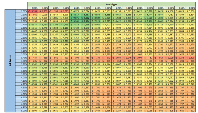
The vast majority of results in this table are positive. With 476 outcomes producing a positive result and only 20 outcomes producing a negative.

The best result is almost $100,000 better if we used triggers of 2.20% and -1.50%.

Conclusion

In the end, what do I make out of all these results? Well to be honest, there is not much I can really do with what I have here. While on individual ETFs they can provide some interesting results, overall there is not really a trend or a pattern emerging, so what has worked in the past for one particular ETF, has not worked in the past for other ETFs.

More importantly, what has worked in the past for one ETF, may not work in the future for the same ETF.

Overall, I do not think this strategy would have any significant benefit, you may get lucky, but unfortunately (or maybe fortunately) it seems that just investing regularly still seems to end up winning the majority of the time.

With all that being said, I will still continue to look to see if there are some adjustments I can make, maybe I can look back further than just the previous day to see if there are any indications of a longer term peak, or a longer term trough that may be able to be taken advantage of.

And once again the statement seems to hold true, time in the market is more important than timing the market. Well, I know it is definitely easier that’s for sure.